bivariate <- lm( # run linear regression
    formula = fthrc ~ faminc, # fthrc = dependent variable, faminc = independent variable
    data = nes
)

modelsummary( # make table of regression results
    bivariate, # with the bivariate regression model from above
    notes = c(
        "Data source: Waffles dataset (McElreath 2020).",
        "Coefficient estimates from OLS.",
        "Standard errors in parentheses" # add a note to tell people how this model was created and with what data.
    ),
    stars = TRUE # print out the stars to show my p-values
)22 Inference and confidence intervals
22.1 What is inference and what does it mean for everything I’ve learned so far?
In the previous exercise we were talking about things like population, sampling, and sample distributions. Why? The motivation for understanding this idea ties back to discussions of statistical significance. When we would say that a regression result was statistically significant, what were we saying? We were saying that, with some pre-specified degree of confidence (usually 95%) that a particular \(\beta\) coefficient or estimate is not equal to 0 (our null hypothesis, \(H_0\)).
In all of our analyses, we are relying on a single sample to test whether there is a relationship between two things. This sample is usually not our population. A sample is just a subset of our population. So how, are we able to make claims about a relationship about a population when we only have data on a single sample? We rely on the central limit theorem and the law of large numbers to help estimate the degree to which we can be sure that any given random sample we have stored on our computer would give us results that are representative of the results we’d get if we were able to run our analysis using data from our whole population.
That is, why we even talk about statistical significance and talk about the probability of the null hypothesis being true given a \(\beta\) coefficient, is because we are almost never able to say that we know there is indeed a non-zero (non-flat) relationship between two variables in the population since we don’t have data on it. Instead, we rely on the assumptions from the central limit theorem to help us make a relatively informed guess about whether these results from a given random sample generalize to the population.
22.2 An example of inference
Let me provide a more concrete example.
The NES dataset contains responses to a survey from just over 1000 adult-aged Americans. Say that I calculate the following bivariate regression to examine whether feelings toward Hillary Clinton are predicted by people’s family income.
| (1) | |
|---|---|
| (Intercept) | 43.643*** |
| (1.218) | |
| faminc | −0.032 |
| (0.035) | |
| Num.Obs. | 1178 |
| R2 | 0.001 |
| R2 Adj. | 0.000 |
| AIC | 11822.2 |
| BIC | 11837.4 |
| Log.Lik. | −5908.086 |
| RMSE | 36.47 |
| + p < 0.1, * p < 0.05, ** p < 0.01, *** p < 0.001 | |
| Data source: Waffles dataset (McElreath 2020). | |
| Credit: damoncroberts.com | |
| Coefficient estimates from OLS. | |
| Standard errors in parentheses |
The particular \(\beta\) coefficient, tells me the effect that family income has on feelings toward Hillary Clinton. This \(\beta\) coefficient is a point estimate that only tells me how positive this relationship is for my sample but not for all adult-aged Americans. So how can I then try to publish a scientific study saying that Americans’ incomes predict support for Hillary Clinton? Using inference I can.
The motivation for calculating the standard errors and things like p-values to determine statistical significance is to help me make claims about whether or not I can be sure that the relationship I’ve calculated in my sample stays that way in the population (of course assuming that my sample is large enough and is random, as per the previous exercises demonstrated). If the p-value is greater than 0.05, we’ve taught you to say that the effect is not statistically significant and if the p-value is less than 0.05, to say that the effect is statistically significant. What this p-value means is that, assuming we have a random sample that is sufficiently large, it is relatively plausible or implausible that if we ran a regression model on our population of adult-aged Americans and had an effect of zero that our sample would’ve given us results like the one we have here.
22.3 Confidence intervals
P-values and the language we use around them is a bit confusing. That last sentence I just wrote out probably makes you have to put your brain in turbo. Trust me, I often do too when I write anything about p-values. Another way that we can present our belief about how likely or unlikely it would be we would have a sample returning results like the one’s we’ve gotten if the actual relationship in the population was zero, is through confidence intervals.
Confidence intervals tell us that if we collected an infinite number of samples – like the one we have on our computer – and ran a regression model on each of them, that we’d expect that the \(\beta\) coefficient we’d calculate with our population would be contained in it 95% of the time. This again, still all assumes that we have a random sample of sufficient size. We are still relying on the central limit theorem here.
Check your understanding
- P-value: The probability that we’d have observed an effect this large or larger if the null hypothesis were true in the population
- Confidence interval: If we took an infinite number of samples, like the one we have on our computer, and estimated a regression for each of those to construct an interval out of those \(\beta\) coefficients, that we’d expect our true relationship in the population to fall within that interval 95% of the time.
So how can we construct a confidence interval and how would we interpret one?
Let’s use the same regression model from before to construct our confidence interval. If we wanted to present our confidence intervals in our table rather than use p-values, we can use the modelsummary() function from the modelsummary package (Arel-Bundock 2022).
bivariate <- lm( # run linear regression
    formula = fthrc ~ faminc, # fthrc = dependent variable, faminc = independent variable
    data = nes
)

modelsummary( # make table of regression results
    bivariate, # with the bivariate regression model from above
    notes = c(
        "Data source: Waffles dataset (McElreath 2020).",
        "Coefficient estimates from OLS.",
        "Standard errors in parentheses" # add a note to tell people how this model was created and with what data.
    ),
    statistic = 'conf.int', # instead of displaying standard errors, do confidence interval
    stars = TRUE # print out the stars to show my p-values
)| (1) | |
|---|---|
| (Intercept) | 43.643*** |
| [41.253, 46.033] | |
| faminc | −0.032 |
| [−0.101, 0.038] | |
| Num.Obs. | 1178 |
| R2 | 0.001 |
| R2 Adj. | 0.000 |
| AIC | 11822.2 |
| BIC | 11837.4 |
| Log.Lik. | −5908.086 |
| RMSE | 36.47 |
| + p < 0.1, * p < 0.05, ** p < 0.01, *** p < 0.001 | |
| Data source: Waffles dataset (McElreath 2020). | |
| Credit: damoncroberts.com | |
| Coefficient estimates from OLS. | |
| Standard errors in parentheses |
If I instead wanted to present the results with a plot, I’ve got a couple of options. The first option would be to use the plotreg() function from the texreg package (Leifeld 2013).
plotreg( # make a plot with the CI's
    bivariate # with the bivariate regression
    ,omit.coef = "(Intercept)" # do not include the intercept term
)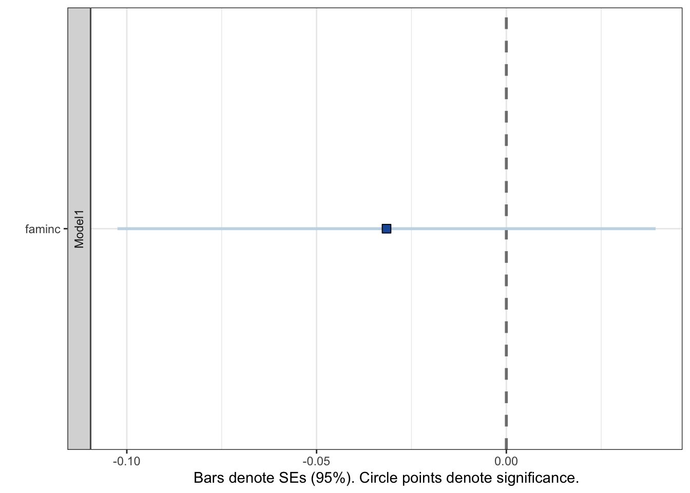
Or I could present the results as a plot with the modelplot() function from the modelsummary package (Arel-Bundock 2022). I personally find this output a bit prettier. It also let’s me use functions from the ggplot2 package (Wickham 2016) like adding notes to the plot and changing the theme! 😎
modelplot( # make a plot with the CI's
    bivariate # with the bivariate regression
    ,coef_omit="Intercept" # do not include the intercept term
) +
geom_vline(
    aes(xintercept = 0),
    linetype = 2
)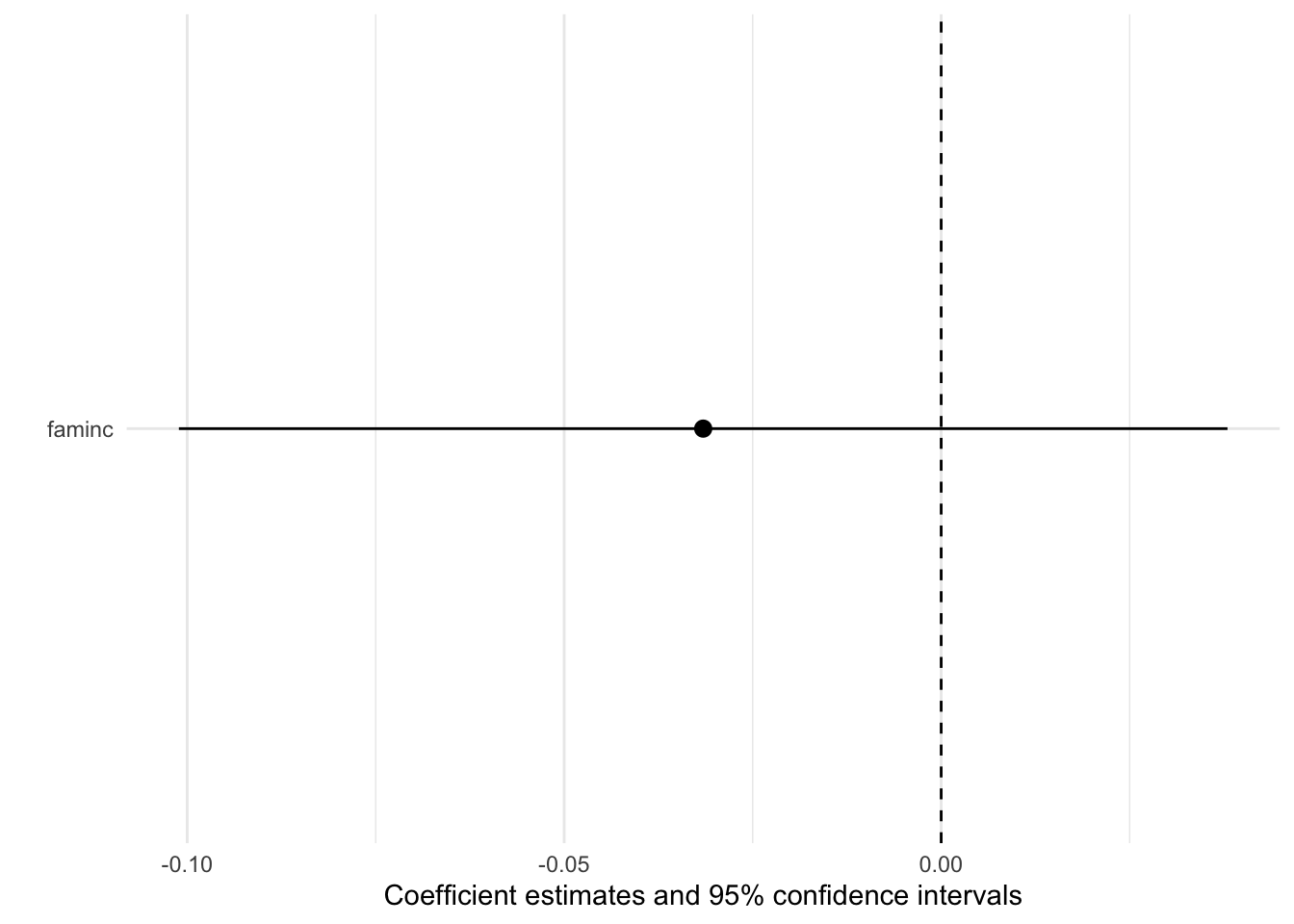
Whether I present these results as a table or by using either of the two packages, I come to similar conclusions: for a unit increase in family income, feelings toward Hillary Clinton decrease by 0.032 units (looked at the table for the specific \(\beta\) coefficient) and this effect is not statistically significant.
How did I know that the effect was not statistically significant by looking at the confidence intervals? Recall, that confidence intervals tell me the 95% of the time if I constructed an interval of all the \(\beta\) coefficients from samples like the one will contain my population parameter. Since my confidence interval overlaps contains 0, there is a chance that 0 is indeed the effect I would observe in my population. If my confidence interval did not contain or overlap with zero, then I could say that the effect was statistically significant because if my true effect in my population were actually zero, there is a less than 5% chance that my confidence interval wouldn’t recognize it – which is a low probability.
All of this will take time to soak in. It is not easy to tie all of these ideas together. You are normal if you are still confused by the idea of inference and statistical significance. The main take away when interpreting confidence intervals is: if the interval contains or overlaps with the value of 0, then your effect is not statistically significant. If the interval does not contain or overlap with the value of 0, then your effect is statistically significant.
22.4 Some final notes
- For a complete working example of this code, go to this page