%%{init: {'theme':'base', 'themeVariables':{'primaryColor':'#ffffff', 'primaryBorderColor': '#000000'}}}%%
graph LR
A[Waffle Houses] --> B[Divorce]
16 🎯Interpreting models with dichotomous independent variables
So far, we’ve talked about linear regression where we estimate and interpret the effect of an independent variable upon a dependent variable. In our interpretation, we’ve treated the independent variable as a continuous one.
Recall that the way that we’ve interpreted a regression output has been to use this template:
For every one unit increase in [my independent variable], I observe a [\(\beta\) coefficient] unit [increase or decrease] in [my dependent variable]. The probability that the effect of [my independent variable] on [my dependent variable] would be this large or larger if the true effect were actually zero is [p-value \(\times 100\)]. It seems relatively [plausible/implausible] that the true effect is not actually zero.
Say that we have an independent variable that is not continuous. In particular, we have an independent variable that is dichotomous – that is to say, a variable that is measured with two categories. We can come up with a number of different examples: is that person’s sex assigned at birth male or female (this is very reductive of a really complex concept, but this is a common example); did this person earn a college degree or not; did they vote in an election or not; there are plenty of examples.
Now say that we use a dichotomous variable, like those above, in a regression model as the independent variable. Would it make sense to use that template above? No, it doesn’t make much sense. What is more intuitive is to interpret the regression results in terms of going from one category to another, what is the increase in the y-variable?
Let’s update our template:
When going from [one category] to [the other category], I observe a [\(\beta\) coefficient] unit [increase or decrease] in [my dependent variable]. The probability that the effect of [my independent variable] on [my dependent variable] would be this large or larger if the true effect were actually zero is [p-value \(\times 100\)]. It seems relatively [plausible/implausible] that the true effect is not actually zero.
That’s really about it!
Let’s look at an example with some code to make it a bit more concrete.
16.1 Example
Let’s go back to my example of the effect of waffle houses on rates of divorce.
# Load packages
library(magrittr) # for pipe operator (%>%)
library(modelsummary) # for table of regression results
library(marginaleffects) # other option for plotting results
library(visreg) # option for plotting results
Let’s say that I have a variable that just tells me: is there a waffle house in the state or not. Not necessarily how many there are. So I want to examine this relationship instead.[^ Though I’d recommend not doing this because you lose a lot of information!]
I, of course, am going to do my normal univariate and bivariate descriptive statistics. Right? I’m just not going to show it here for the purposes of brevity. Now, let’s say that after I’ve done those things, I want to run my regression. I can run the code as usual, with one slight tweak with my regression model.
regression <- lm( # run a linear regression
    formula = Divorce ~ I(WaffleHousesBinary), # Divorce is predicted by a binary version of my wafflehouses variable
    data = waffles_clean # using this dataset
)

modelsummary(
    regression, # make a table summarizing results of my regression
        notes = c(
        "Data source: Waffles dataset (McElreath 2020).",
        "Coefficient estimates from OLS.",
        "Standard errors in parentheses" # add a note to tell people how this model was created and with what data.
    ),
    stars = TRUE # print out the stars to show my p-values
)| (1) | |
|---|---|
| (Intercept) | 8.996*** |
| (0.340) | |
| I(WaffleHousesBinary)Yes | 1.384** |
| (0.480) | |
| Num.Obs. | 50 |
| R2 | 0.147 |
| R2 Adj. | 0.130 |
| AIC | 198.8 |
| BIC | 204.6 |
| Log.Lik. | −96.420 |
| RMSE | 1.66 |
| + p < 0.1, * p < 0.05, ** p < 0.01, *** p < 0.001 | |
| Data source: Waffles dataset (McElreath 2020). | |
| Coefficient estimates from OLS. | |
| Standard errors in parentheses |
When going from states without a waffle house to states with a waffle house, I observe a 1.3 unit increase in state divorce rate. The probability that the effect of waffle houses on divorce rate would be this large or larger if the true effect were actually zero is 1.384. It seems relatively plausible that the true effect is not actually zero.
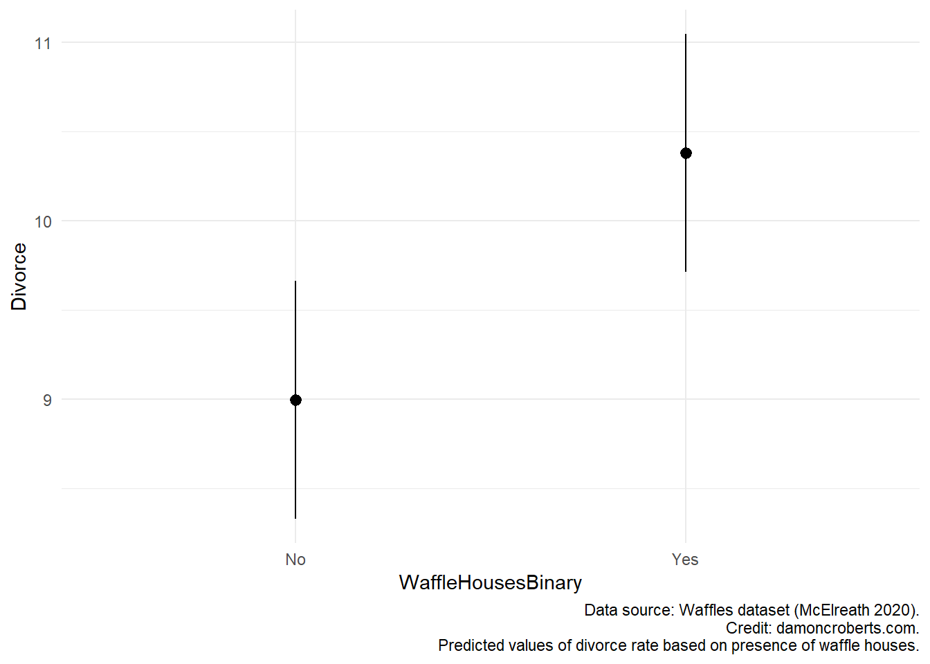
I can plot the predicted values I would get for each value of the WaffleHouses dataset using the marginaleffects package. I can use the following code to produce Figure 16.2. What this shows me is that states that do have waffle houses have higher rates of divorce. The dots tell me what the estimated value of divorce would be for states that do not have a waffle house and ones that do based on my regression model. The bars, represent the amount of uncertainty that I have from my model. Just as the table of my regression demonstrates (Table 16.1), these effects are statistically significant. The bars do not overlap on this plot which shows that I am sure, to some degree, that rates of divorce are indeed influenced by the presence of a waffle house.
plot_predictions( # plot the predictions
    regression, # use the regression model
    by = "WaffleHousesBinary" # should be split up by whether there is a waffle house or not
) +
theme_minimal() + # add this theme to the plot
labs( # add these labels
    caption = "Data source: Waffles dataset (McElreath 2020).\n Predicted values of divorce rate based on presence of waffle houses."
)
marginaleffects packageI could also use the visreg package to show me differences in expectations about rates of divorce based on states that do versus states that do not have waffle houses.
visreg( # plot the results of the model
    regression, # of my regression model
    "WaffleHousesBinary", # what is the variable it should be split by?
    band = FALSE, # do not include band of uncertainty
    overlay = TRUE # include an overlay
)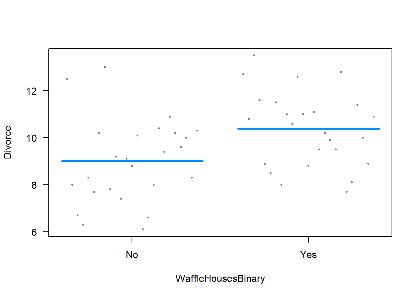
Now, this looks different than what Dr. Philips has. Why? Well, I am only doing a bivariate regression. My X-axis does not have a continuous variable. So, things will look a bit funky as a result.
In general, though, both plots show us pretty much the same thing. That states with waffle houses have higher divorce rates than states that do not have waffle houses.
16.2 Some final notes
- For a complete working example of this code, go to this page