17 🫠 When we think our effect may be conditional on something else

Nuance Spongebob GIFfrom Nuance GIFs

So far, we have examined how one variable may have an effect on another and we have examined how we think a confounding variable may be partially explaining the relationship we are primarily interested in.

With confounding variables, we are concerned about the fact that it often explains both the independent and dependent variables. Remember, we discussed how that feature often causes problems for giving us really imprecise estimates of the effect that the independent variable has on our dependent variable.

Well, there is another sort of relationship we may be interested in examining. We may be interested in not just how the independent variable effects the dependent variable, but we may think that the relationship between our independent variable and dependent variable is dependent or conditional on something else. That is, the relationship between the independent and dependent variable is not the same across some groups we might be interested in.

Let’s think of a couple of examples:

Say that we are interested in examining the relationship between someone’s Ideology and Vote Choice. Well, we may think that that relationship exists, BUT that that relationship may appear different between Black and White people. That is, the relationship between Ideology and Vote Choice between White folks may be stronger than it would be for Black folks. Why might we think that? Well, there is lot’s of really wonderful research out there that you should check out on this topic!! For starters, check out this book. It is perhaps one of my most favorite!
Say that we think that there is a relationship between someone’s income and support for Donald Trump in the 2016 presidential election. Seems reasonable enough. But we may expect that this relationship is “moderated” or is conditional upon whether that person identifies as female or male. That is, we may expect that the effect of income on Trump votes in 2016 looks different for women than it would men.

We can think of plenty of other examples! And a lot of modern political science is often involved in looking more into these sorts of theories as opposed to the more simple ones like ideology predicting vote choice. Examining these relationships provides quite a lot more nuance to our theories of how politics works.

So how do we examine these relationships? Well, the code is actually quite straight-forward. The interpretation… not so much unfortunately. I’d highly recommend checking out Dr. Philip’s slides and RScripts on interactions for extra help with this. The most important thing is to understand the intuition behind what we are doing with an interaction model. The types of questions I posed in the examples above depict such an intuition. It isn’t that we think that our independent variable predicts our dependent variable. It is that we think this relationship exists, but it looks different based on what value we are looking at for some other variable. An interaction term is not necessarily a confounder. Do not confuse those!.

So, let’s go through the code on this.

Say I want to examine the effect of someone’s income on someone’s feelings toward Hillary Clinton (higher values means that they like Clinton more, and lower values means they like Clinton less). However, I think that this relationship is dependent on someone’s gender. That is, just because someone has a higher income, it doesn’t mean that high income men and high income women will similarly like Clinton.

library(magrittr) # for pipe operator (%>%)
library(modelsummary) # for making regression tables
library(marginaleffects) # for making plots of results
library(visreg) # alternative for making plots of results

Say I have already run all of my univariate and bivariate descriptive statistics. Now I can start to examine a regression. I start with a bivariate regression which I present in Table 22.1.

bivariate <- lm( # run linear regression
    formula = fthrc ~ faminc, # fthrc = dependent variable, faminc = independent variable
    data = nes
)

modelsummary( # make table of regression results
    bivariate, # with the bivariate regression model from above
    notes = c(
        "Data source: Waffles dataset (McElreath 2020).",
        "Coefficient estimates from OLS.",
        "Standard errors in parentheses" # add a note to tell people how this model was created and with what data.
    ),
    stars = TRUE # print out the stars to show my p-values
)

Table 17.1: The effect of family income on feelings toward Hillary Clinton
	(1)
(Intercept)	43.643***
	(1.218)
faminc	−0.032
	(0.035)
Num.Obs.	1178
R2	0.001
R2 Adj.	0.000
AIC	11822.2
BIC	11837.4
Log.Lik.	−5908.086
RMSE	36.47
+ p < 0.1, * p < 0.05, p < 0.01, * p < 0.001
Data source: Waffles dataset (McElreath 2020).
Credit: damoncroberts.com
Coefficient estimates from OLS.
Standard errors in parentheses

For every unit increase in family income, I would expect a -0.032 decrease in favorable attitudes directed toward Hillary Clinton. The probability that the effect of family income on feelings toward Hillary Clinton would be this large or larger if the true effect were actually 0 is 37.336. It seems relatively plausible that the effect of income on feelings toward Hillary Clinton is actually zero.

Now, let’s examine how this relationship between family income and feelings toward Hillary Clinton is different depending on whether we look at folks who identify as Female or Male.

interaction <- lm( # run linear regression
    formula = fthrc ~ faminc + gender + faminc:gender, # fthrc = dependent variable, faminc = independent variable
    data = nes
)

modelsummary( # make table of regression results
    interaction, # with the interaction regression model from above
    notes = c(
        "Data source: Waffles dataset (McElreath 2020).",
        "Coefficient estimates from OLS.",
        "Standard errors in parentheses" # add a note to tell people how this model was created and with what data.
    ),
    stars = TRUE # print out the stars to show my p-values
)

Table 17.2: The effect of family income on feelings toward Hillary Clinton, conditional on gender.
	(1)
(Intercept)	40.746***
	(1.749)
faminc	−0.069
	(0.053)
genderFemale	5.702*
	(2.429)
faminc × genderFemale	0.063
	(0.071)
Num.Obs.	1178
R2	0.010
R2 Adj.	0.007
AIC	11815.2
BIC	11840.6
Log.Lik.	−5902.616
RMSE	36.30
+ p < 0.1, * p < 0.05, p < 0.01, * p < 0.001
Data source: Waffles dataset (McElreath 2020).
Credit: damoncroberts.com
Coefficient estimates from OLS.
Standard errors in parentheses

Here’s what I see. When I am looking at male respondents (when family income equals zero), for every unit increase in family income, there is a -0.069 unit decrease in feelings toward Hillary Clinton. This effect does not appear statistically insignificant. When Looking at Female individuals with zero income, they tend to report 5.702 points higher on their feelings toward Hillary Clinton relative to Males with zero income. This does not appear to be statistically significant. We see that for every unit increase in family income, Women tend to report 0.063 points higher on their feelings toward Hillary Clinton relative to males. This effect also does not appear to be statistically significant.

Let’s visualize what this table is communicating.

We can use either visreg or the marginaleffects packages to help us with this.

plot_predictions( # plot predicted values from this
    interaction, # plot the interaction model
    condition = c("faminc", "gender")
) +
theme_minimal() +
labs(
    y = "Feeling thermometer: Hillary Clinton",
    x = "Family income",
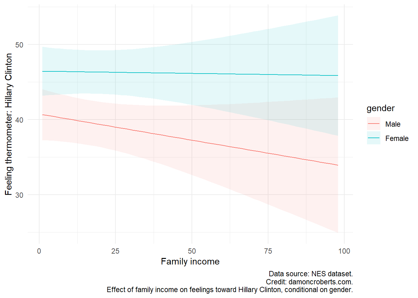
    caption = "Data source: NES dataset.\n Effect of family income on feelings toward Hillary Clinton, conditional on gender."
)

Figure 17.1: Effect of family income on attitudes toward Hillary Clinton, conditional on gender

visreg(# plot the predicted values from this
    interaction,
    "faminc",
    by = "gender",
    band = FALSE,
    overlap = TRUE
)

Figure 17.2: Effect of family income on attitudes toward Hillary Clinton, conditional on gender

What do both of these plots tell us? Well, first we can see that, for Males, there is a decrease in reported attitudes toward Hillary Clinton as one’s family income increases. We can also see that Female respondents reported more positive attitudes toward Hillary Clinton than Male respondents, overall. However, we see that as Female respondents’ income increases, their attitudes toward Hillary Clinton do not increase all that much. So, we come to the same conclusions as we did with the table! Different ways to communicate similar information.

Interpreting interaction models are really hard. Just make sure that you try to understand the intuition or the motivation behind why we’d want to do one in the first place. Taking that first step will make the interpretation of these models much easier!

17.1 Some final notes

For a complete working example of this code, go to this page