So far we have been using ordinary least squares regression (OLS) to examine the causal relationship between two variables. As we have discussed, OLS is a really powerful tool for this purpose and many applied statisticians use it for a lot of their work. While it is a great general tool, like many general tools, it has its limitations and we often times need to use more refined tools to account for such limitations.
Let’s see what happens when we try to fit a OLS regression with a dichotomous (two category) dependent variable. For this example, I am going to examine the relationship between how someone voted in the 2012 Presidential election and their partisan affiliation. So let me run a simple bivariate linear regression. This model will be what is called a Linear Probability Model. The underlying math between OLS and LPM’s remain the same. What changes, however, is that the dependent variable being dichotomous in this case leads to differences in interpretation and have other underlying implications for the model.
First, I am going to recode the vote12 variable to contain two categories: did they vote for Romney or Obama? Anyone who was not asked the question or reported voting for someone else are coded as NA (missing) values. I am also going to recode pid7 to make those who said “Not Sure” to be marked as “Independents” and to then convert it into integers rather than as a factor variable.
# make a new column called vote_obama...#* ...and make the default value NAnes$vote_obama <-NA# if voted for Romney, give the new column a value of 0nes$vote_obama[nes$vote12 =="Mitt Romney"] <-0# if voted for Obama, give the new column a value of 1nes$vote_obama[nes$vote12 =="Barack Obama"] <-1# Check to make sure everything looks rightsummary(nes$vote12)
   Min. 1st Qu.  Median    Mean 3rd Qu.    Max.    NA's
 0.0000  0.0000  1.0000  0.5811  1.0000  1.0000     309
# make a new column called pid7_int...#* ...and make the default value NAnes$pid7_int <-NA# if said "Not sure", make them a independentnes$pid7[nes$pid7 =="Not sure"] <-"Independent"# then remove labels from pid7 and store as pid7_intnes$pid7_int <-as.numeric(nes$pid7)# Make a new column called white...#* ...and make the default value NAnes$white <-NA# if said "White", then make them Whitenes$white[nes$race =="White"] <-"White"# if said "Black", then make them Blacknes$white[nes$race =="Black"] <-"Black"# Convert to factornes$white <-as.factor(nes$white)# let's remove all NA rows from the datasetnes_clean <-na.omit(nes)
# Run linear regressionbivariate_linear <-lm(formula = vote_obama ~ pid7_int # does party identification predict vote choice? , data = nes_clean)# Make a table of resultsmodelsummary( bivariate_linear # the regression I made above , notes =c("Data source: NES dataset." , "Estimates from an Ordinary Least Squares regression." , "Standard errors in parentheses." ) # include these notes at the bottom of the table , stars =TRUE# include stars in table , output ="my_linear_bivariate_regression.docx")
Table 24.1: The effect of party identification on support for Obama
(1)
(Intercept)
1.194***
(0.021)
pid7_int
−0.175***
(0.005)
Num.Obs.
746
R2
0.628
R2 Adj.
0.627
AIC
336.9
BIC
350.8
Log.Lik.
−165.469
RMSE
0.30
+ p < 0.1, * p < 0.05, ** p < 0.01, *** p < 0.001
Data source: NES dataset.
Credit: damoncroberts.com
Estimates from an Ordinary Least Squares regression.
Standard errors in parentheses.
Since the dependent variable is dichotomous, my interpretation is going to be slightly different. Now it tells me that the stronger I identify with Republicans, the probability that I voted for Obama decreases by 0.173 points. This effect is statistically significant.
For each unit increase in [my independent variable], the probability of [the 1 category] [increases/decreases]. The effect [is/is not] statistically significant. Which means that it is relatively [implausible/plausible] that I would have estimated an effect that large or larger if there was truly no relationship between the variables.
Let’s see whether this model was a good one, though. We might first believe that there are confounding variables that I have missed. The most obvious one would be that I had excluded race and I should fit a multivariate regression controlling for that.
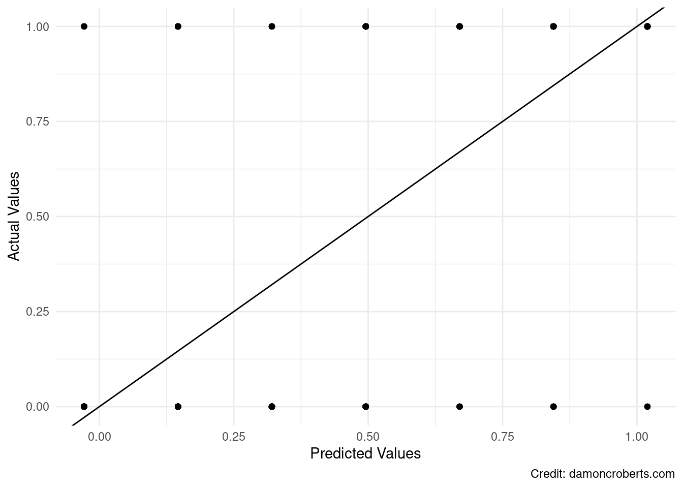
However, there are some other things that are lurking here. Let’s look at the predicted and actual values here.
# make a table (data.frame) with predicted and actual valuespredicted_plot <-data.frame(predicted_values =predict(bivariate_linear),actual_values = nes_clean$vote_obama)#plot predicted vs. actual valuesggplot(data = predicted_plot # take the data from predicted_plot) +geom_point( # put points on the graph based on the dataaes(x = predicted_values, # put predicted_values column on x-axisy = actual_values # put actual_values column on y-axis )) +geom_abline( # draw a line through the pointsintercept=0 , slope=1) +theme_minimal() +# make it prettier with this themelabs( # add labels to the plotx='Predicted Values' , y='Actual Values')
Figure 24.1: Predicted values versus actual values
There are a few things that stand out here: 1. I am predicting lots of values that do not exist. In my variable, you either voted for Obama or you didn’t. The model predicts that there are people that are between that. The model can also predict that there are people that are above the value of 1 (voted for Obama) and below 0 (did not vote for Obama). These are not possible values and they make no sense. 2. I have some really massive residuals (difference between my predicted values and my actual values) in some areas but not in others. This leads to me having an unequal variance in my error term. Which as we discussed last week is a problem. To show that this is the case, I can use some of the model diagnostics from last week to prove it.
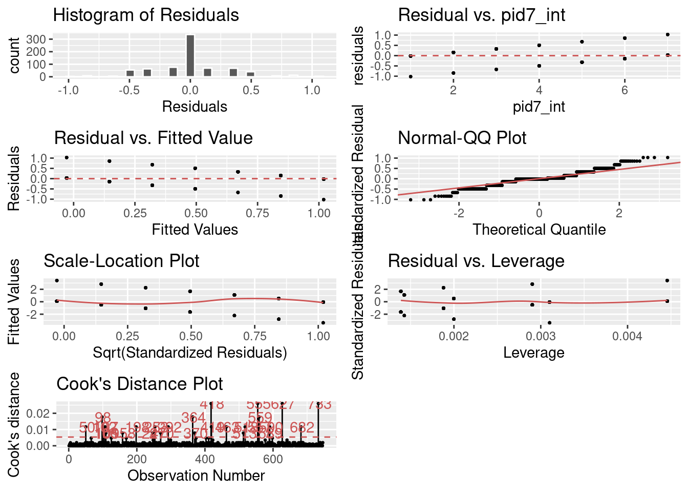
gg_diagnose( bivariate_linear)
Figure 24.2: Diagnostics of LPM
Look at all of those plots – look at them! They are bad. I’ve got lots of instances with a residual of 0, but look at the variance on those residuals! To see that I can look at my Normal-QQ plot which looks problematic and so does my Cook’s distance plot (remember, for this plot I do not want spikes to show up in clusters).
So how can we address these problems created by the LPM? We can estimate a model that is designed to handle dichotomous dependent variables. This model is called the logistic regression model (sometimes called logit).
How do logistic regression models work? Well, it is relatively complex. But, what you should know is that it operates much the same way an OLS does. The big difference that you should be aware of is that we can improve upon the LPM model by ensuring that our predicted values can either be 0 or 1. This solves those two issues that we had prior. How does the LPM do this? It uses what is called a link function. Specifically, it uses a log-link function:
Where \(P_1\) is the probability of vote_obama being equal to 1. What is different here is that now the relationship between our \(\beta\) coefficients and our \(\hat{Y}\) values is no longer 1 to 1. What this means is that the way that we interpret the effect of our independent variables can no longer be stated as: “a one unit increase in our independent variable leads to a \(\beta\) unit increase in our dependent variable”. Instead, the link function means that the relationship is in terms of logged-odds. So the interpretation is now “a one unit increase in our independent variable leads to a logged-odds unit increase in the probability of our dependent variable being equal to one.”
Without going too much into the algebra of this, this relatively simple link function does quite a lot to solve our problems that we get with the LPM! Let me show you!
Using the glm() function, we can run this logistic regression model.
# run logistic regression modellogistic_regression <-glm(formula = vote_obama ~ pid7_int # vote for obama as predicted by party identification , data = nes_clean # using this dataset , family = binomial # a logistic regression model)# make table of resultsmodelsummary( logistic_regression # the regression I made above , notes =c("Data source: NES dataset." , "Estimates from an Ordinary Least Squares regression." , "Standard errors in parentheses." ) # include these notes at the bottom of the table , stars =TRUE# include stars in table , output ="my_linear_bivariate_regression.docx")
Table 24.2: The effect of party identification on vote choice
(1)
(Intercept)
5.256***
(0.374)
pid7_int
−1.306***
(0.090)
Num.Obs.
746
AIC
430.4
BIC
439.6
Log.Lik.
−213.199
RMSE
0.29
+ p < 0.1, * p < 0.05, ** p < 0.01, *** p < 0.001
Data source: NES dataset.
Credit: damoncroberts.com
Estimates are from a logistic regression; interpreted as logged-odds.
Standard errors in parentheses.
How would we interpret the main part of the table we are interested in? The closer to a strong Republican you become, the logged-odds of voting for Obama decreases by 1.258 units. This effect is statistically significant.
But what the heck does it mean for the logged-odds to decrease? Really hard for us to conceptualize that. At least it is much harder than a one unit change leading to a \(\beta\) unit change like we had with OLS. The second equation above shows us that the link function is essentially the natural log of the odds. So we can calculate the odds ratio by exponentiating the coefficient.
Remember that we can look inside our objects by using the str() function:
From this output I want to grab a coefficient and specifically the second coefficient. Then once I have it, I’ll take the exponent of it!
exp(logistic_regression$coefficients[2])
 pid7_int
0.2708807
The output is 0.284. This means that the odds ratio of voting for Obama the closer someone is to a strong Republican, is 0.284. For those that are familiar with odds, this might make sense. For the rest of us, we still might be a bit confused. An odds ratio of 1 would mean that I am neither more or less likely to vote for Obama. Since I am below that, it would mean that the odds of me voting for Obama the more Republican I become decrease by 71.6% (1 - 0.284).
As a shortcut, the modelsummary package lets me display my results in terms of odds ratios by including one extra option!
# make table of resultsmodelsummary( logistic_regression # the regression I made above , exponentiate =TRUE# show odds ratio instead , notes =c("Data source: NES dataset." , "Credit: damoncroberts.com" , "Estimates are from a logistic regression; interpreted as odds ratios." , "Standard errors in parentheses." ) # include these notes at the bottom of the table , stars =TRUE# include stars in table , output ="odds_ratio_results.docx")
Table 24.3: The odds-ratio of voting for Obama based on your party identification
(1)
(Intercept)
191.787***
(71.814)
pid7_int
0.271***
(0.024)
Num.Obs.
746
AIC
430.4
BIC
439.6
Log.Lik.
−213.199
RMSE
0.29
+ p < 0.1, * p < 0.05, ** p < 0.01, *** p < 0.001
Data source: NES dataset.
Credit: damoncroberts.com
Estimates are from a logistic regression; interpreted as odds ratios.
Standard errors in parentheses.
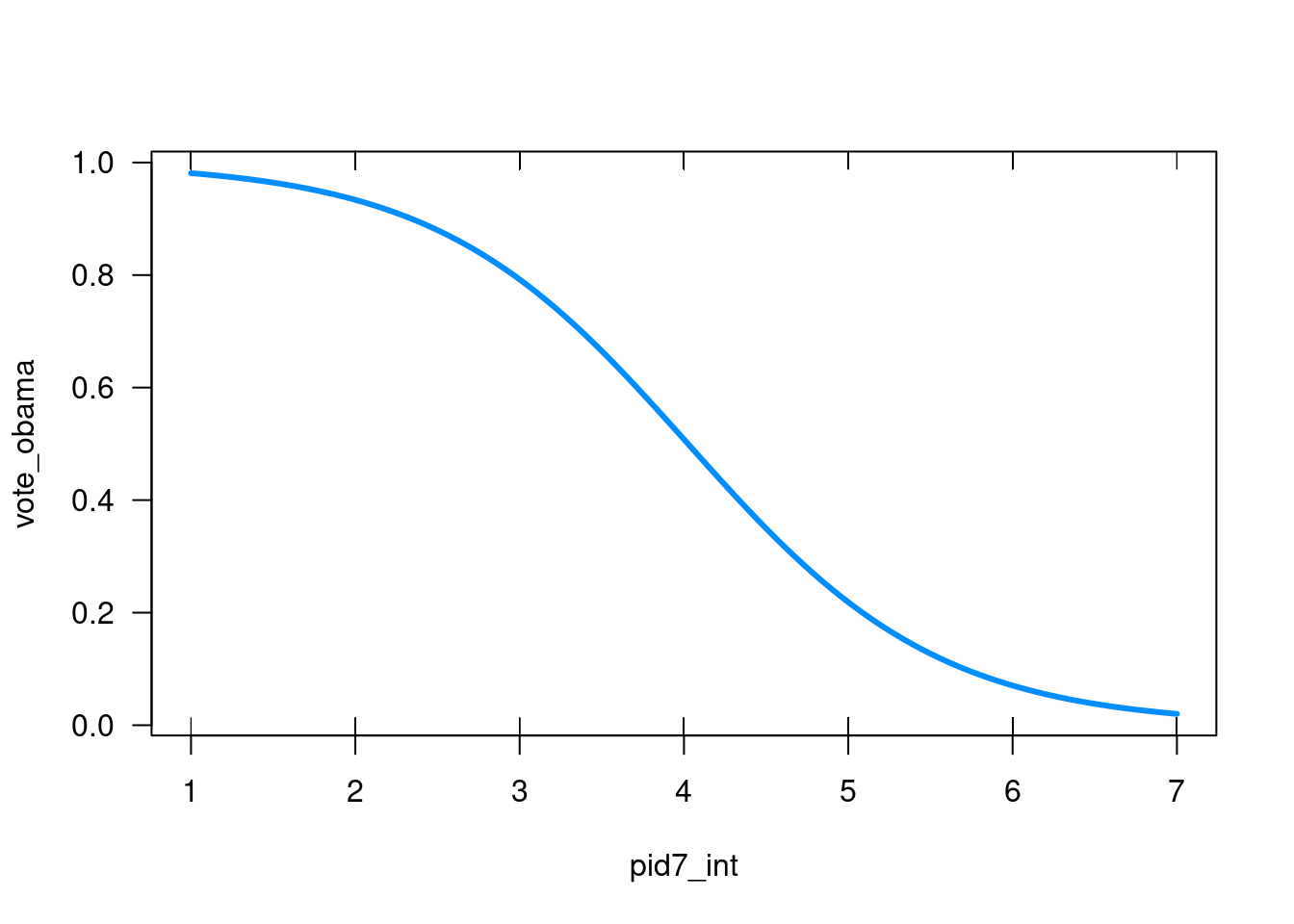
One option would be to use the visreg package (Breheny and Burchett 2017) to plot those predicted probabilities:
visreg( logistic_regression # the logistic regression model above , "pid7_int"# the independent variable , scale ="response"# want to look at it in terms of possible values (0 or 1) , band =FALSE# do not show a band of confidence intervals)
Figure 24.3: The predicted probability of voting for Obama (Visreg)
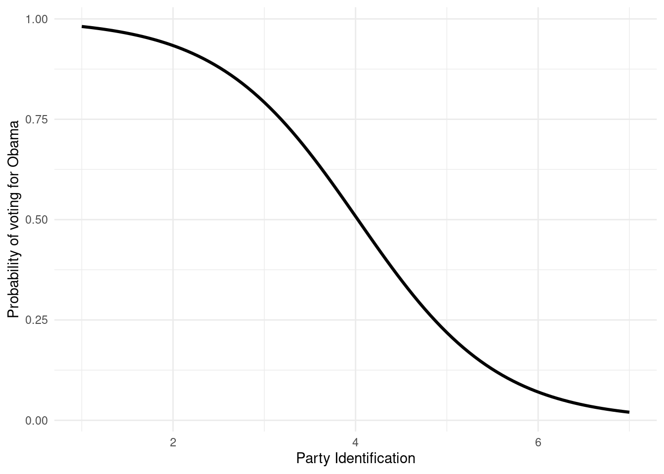
Or, I can use the jtools package (Long 2022) to make a plot of my predicted probabilities using the ggplot2 package (Wickham 2016) as a backend. This means that I can make adjustments to this plot the way I would with my other plots using ggplot2. Nice!
effect_plot( logistic_regression # use the results from this model , pred = pid7_int # the independent variable to look at , interval =FALSE# do not show confidence interval) +theme_minimal() +# apply the minimal themelabs( # apply the following labelsy ="Probability of voting for Obama" , x ="Party Identification")
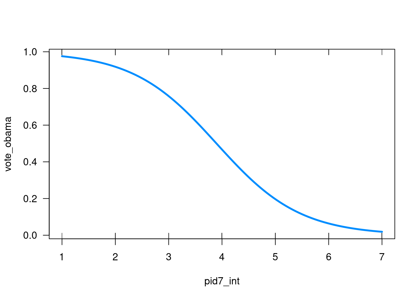
Figure 24.4: Predicted probability of voting for Obama depending on party identification
Both plots show me the same thing: The probability that I’d vote for Obama, the more Republican I am decreases. We see that the probability of voting for Obama if I am a strong Democrat is almost 1. However, if I am an independent, the probability that I vote for Obama is just above 0.5. And if I am a strong Republican, the probability that I vote for Obama is just above 0.
While the interpretation of these models requires a bit more work, we can see that we are no longer coming up with super wonky predictions (value outside of 0 and 1). Because we don’t have really weird predictions anymore, we can also be a bit more comfortable that our residuals aren’t super messed up anymore either!
Now, say that I do a multivariate logistic regression. The interpretation of this plot changes slightly and can be a bit more complicated!
# run logistic regression modellogistic_regression <-glm(formula = vote_obama ~ pid7_int + white # vote for obama as predicted by party identification and race , data = nes_clean # using this dataset , family = binomial # a logistic regression model)# make table of resultsmodelsummary( logistic_regression # the regression I made above , notes =c("Data source: NES dataset." , "Estimates from an Ordinary Least Squares regression." , "Standard errors in parentheses." ) # include these notes at the bottom of the table , stars =TRUE# include stars in table , output ="my_linear_bivariate_regression.docx")
Table 24.4: The effect of party identification on vote choice
(1)
(Intercept)
7.892***
(0.893)
pid7_int
−1.275***
(0.091)
whiteWhite
−2.924***
(0.794)
Num.Obs.
746
AIC
409.8
BIC
423.6
Log.Lik.
−201.888
RMSE
0.28
+ p < 0.1, * p < 0.05, ** p < 0.01, *** p < 0.001
Data source: NES dataset.
Credit: damoncroberts.com
Estimates are from a logistic regression; interpreted as logged-odds.
Standard errors in parentheses.
visreg( logistic_regression # the logistic regression model above , "pid7_int"# the independent variable , scale ="response"# want to look at it in terms of possible values (0 or 1) , band =FALSE# do not show a band of confidence intervals)
Figure 24.5: The predicted probability of voting for Obama (Visreg)
This plot demonstrates that the probability of voting for Obama decreases the more Republican an individual is when holding the white variable at it’s mean value.
What if we don’t want to hold white at it’s mean value? Well we can plot this with a few tweaks to the function.
summary(nes_clean$white)
Black White
  104   642
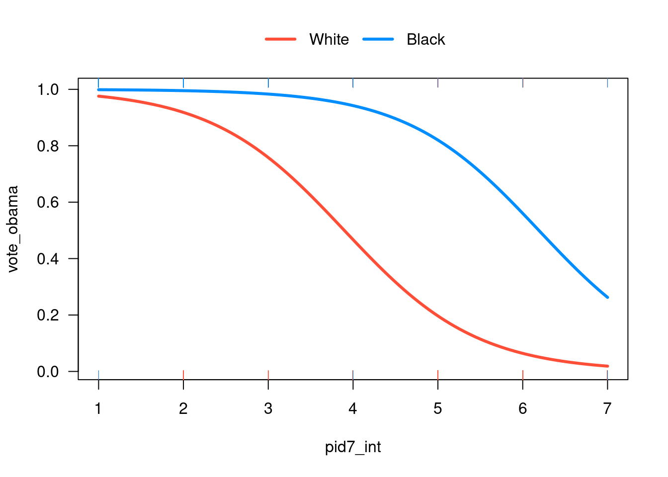
visreg( logistic_regression # the logistic regression model above , "pid7_int"# the independent variable , by ="white" , breaks =c("White", "Black") , scale ="response"# want to look at it in terms of possible values (0 or 1) , band =FALSE# do not show a band of confidence intervals , overlay =TRUE# overlay the plots)
Figure 24.6: Predicted probability of voting for Obama depending on party identification
This plot demonstrates that the probability of voting for Obama decreases the more Republican someone is. We see this occurs for both white and Black respondents. Though it appears that the decrease in predicted probability for Obama for Black respondents remains relatively high, even if they identify as a “Strong Republican”.
Note you can make a similar graph using the effect_plot() function.
24.1 Some final notes:
OLS when run with a dichotomous dependent variable is called the LPM model.
Problems with the LPM model:
Impossible predicted values for our dependent variable.
Heteroskedastic errors (unequal variance in our residuals)
Logistic regression:
Fixes the problems with the LPM model
More work to interpret them/harder to interpret
For an R script to replicate what we did in this exercise, go to this page.
Breheny, Patrick, and Woodrow Burchett. 2017. “Visualization of Regression Models Using Visreg.”The R Journal 9 (2): 56–71.